PRINCIPLES OF ENVIRONMENTAL TOXICOLOGY AND CONTAMINATION (PART II)

Table of Contents

1. Index
2. UNIT 5 - Transport and fate of contaminants in the environment
   1. Introduction
   2. Transport processes
   3. Environmental persistence and transformation processes
   4. Bioaccumulation
   5. Environmental fate models
   6. Brief conclusion
3. UNIT 6 - Principles of toxicokinetics and toxicodynamics
4. UNIT 7 - Biotransformation
5. UNIT 8 - Toxicity Testing
6. Glossary of key terms associated with environmental toxicology

Environmental fate models

A qualitative introduction to the transport and fate of chemicals in the environment is made above. The aim of most engineers and fate chemists is to translate this qualitative picture into a conceptual model and ultimately into a quantitative description that can be used to reconstruct or predict the fate of a chemical in the environment (Fig. 1). This quantitative description generally takes the form of a mass balance model. The plan is to compartmentalize the environment into defined units (i.e., control volumes) and to write a mathematical expression for the mass balance within the compartment. The transfer between compartments can be included as the complexity of the model increases. It is necessary to take into account that there is a large deal of subjectivity to assembling a mass balance model. Nevertheless, each decision to exclude or include a compartment or process is based on one or more assumptions. Most of these assumptions can be tested at some level. Over time, the applicability of different assumptions for environmental conditions and particular chemicals becomes known and model standardization becomes possible. For the construction of a mass balance model, it is necessary:

1^st - To define the spatial and temporal scales to be considered and to establish the environmental compartments or control volumes;
2^nd- To identify and quantify the source emissions;
3^rd - To write the mathematical expressions for advective and diffusive transport processes;
4^th - To quantify the chemical transformation processes.

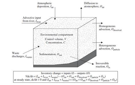
This model-building process is illustrated in Figure 5.

In figure 5, the change in chemical inventory (total mass in the system) was simply equated with the difference between chemical inputs and outputs to the system. The inputs could include several point and nonpoint sources or could be a single estimate of total chemical load to the system. The outputs include all of the loss mechanisms: irreversible transformation reactions and transport out of the compartment. If steady state can be assumed (i.e., the concentration of the chemical in the compartment is not changing over the timescale of the model), the inventory change is zero and we have a simple mass balance equation to solve. On the other hand, unsteady-state conditions would require a numerical solution to the differential equations.

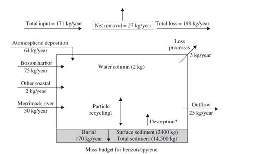
There are many tricks and shortcuts to this process. It is usually prudent to start with estimates of chemical half-lives in air, water, soil, and sediment and to perform a sensitivity analysis with the model to determine which processes are most important. An illustration of this mass balance approach for benzo[a]pyrene is depicted in Figure 6. This approach allows a first-order evaluation of how chemicals enter in the environment, what happens to them in the environment, and what the exposure concentrations will be in different environmental media. As a conclusion, the chemical mass balance provides essential information to contaminant exposure in both humans and wildlife.

Additional information about environmental fate models can be found in the following articles and links:

http://www.socopse.se/decisionsupportsystem/tools/environmentalfatemodeling.4.3d9ff17111f6fef70e9800053707.html

http://www.socopse.se/decisionsupportsystem/tools/quickguidetoenvironmentalfatemodels.4.3d9ff17111f6fef70e9800068582.html

http://www.itopf.com/knowledge-resources/documents-guides/fate-of-oil-spills/oil-spill-modelling/

http://www.arcopol.eu/